Perform SLAM Using 3-D Lidar Point Clouds
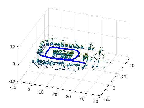
This example demonstrates how to implement the simultaneous localization and mapping (SLAM) algorithm on collected 3-D lidar sensor data using point cloud processing algorithms and pose graph optimization. The goal of this example is to estimate the trajectory of the robot and create a 3-D occupancy map of the environment from the 3-D lidar point clouds and estimated trajectory.
The demonstrated SLAM algorithm estimates a trajectory using a Normal Distribution Transform (NDT) based point cloud registration algorithm and reduces the drift using SE3 pose graph optimization using trust-region solver whenever a robot revisits a place.
Load Data And Set Up Tunable Parameters
Load the 3-D lidar data collected from a Clearpath™ Husky robot in a parking garage. The lidar data contains a cell array of n-by-3 matrices, where n is the number 3-D points in the captured lidar data, and the columns represent xyz-coordinates associated with each captured point.
outputFolder = fullfile(tempdir,'ParkingLot');

dataURL = ['https://ssd.mathworks.com/supportfiles/lidar/data/' ...
            'NatickParkingLotLidarData.tar'];

pClouds = helperDownloadData(outputFolder,dataURL);
Parameters For Point Cloud Registration Algorithm
Specify the parameters for estimating the trajectory using the point cloud registration algorithm. maxLidarRange specifies the maximum range of the 3-D laser scanner.
maxLidarRange = 20;
The point cloud data captured in an indoor environment contains points lying on the ground and ceiling planes, which confuses the point cloud registration algorithms. Some points are removed from the point cloud with these parameters:
referenceVector- Normal to the ground plane.maxDistance- Maximum distance for inliers when removing the ground and ceiling planes.maxAngularDistance- Maximum angle deviation from the reference vector when fitting the ground and ceiling planes.
referenceVector = [0 0 1];
maxDistance = 0.5;
maxAngularDistance = 15;
To improve the efficiency and accuracy of the registration algorithm, the point clouds are downsampled using random sampling with a sample ratio specified by randomSampleRatio.
randomSampleRatio = 0.25;
gridStep specifies the voxel grid sizes used in the NDT registration algorithm. A scan is accepted only after the robot moves by a distance greater than distanceMovedThreshold.
gridStep = 2.5;
distanceMovedThreshold = 0.3;
Tune these parameters for your specific robot and environment.
Parameters For Loop Closure Estimation Algorithm
Specify the parameters for the loop closure estimation algorithm. Loop closures are only searched within a radius around the current robot location specified by loopClosureSearchRadius.
loopClosureSearchRadius = 3;
The loop closure algorithm is based on 2-D submap and scan matching. A submap is created after every nScansPerSubmap (Number of Scans per submap) accepted scans. The loop closure algorithm disregards the most recent subMapThresh scans while searching for loop candidates.
nScansPerSubmap = 3;
subMapThresh = 50;
An annular region with z-limits specified by annularRegionLimits is extracted from the point clouds. Points outside these limits on the floor and ceiling are removed after the point cloud plane fit algorithms idenfity the region of interest.
annularRegionLimits = [-0.75 0.75];
The maximum acceptable Root Mean Squared Error (RMSE) in estimating relative pose between loop candidates is specified by rmseThreshold. Choose a lower value for estimating accurate loop closure edges, which has a high impact on pose graph optimization.
rmseThreshold = 0.26;
The threshold over scan matching score to accept a loop closure is specified by loopClosureThreshold. Pose Graph Optimization is called after inserting optimizationInterval loop closure edges into the pose graph.
loopClosureThreshold = 150;
optimizationInterval = 2;
Initialize Variables
Set up a pose graph, occupancy map, and necessary variables.
% 3D Posegraph object for storing estimated relative poses
pGraph = poseGraph3D;
% Default serialized upper-right triangle of 6-by-6 Information Matrix
infoMat = [1,0,0,0,0,0,1,0,0,0,0,1,0,0,0,1,0,0,1,0,1];
% Number of loop closure edges added since last pose graph optimization and map refinement
numLoopClosuresSinceLastOptimization = 0;
% True after pose graph optimization until the next scan
mapUpdated = false;
% Equals to 1 if the scan is accepted
scanAccepted = 0;

% 3D Occupancy grid object for creating and visualizing 3D map
mapResolution = 8; % cells per meter
omap = occupancyMap3D(mapResolution);
Preallocate variables for the processed point clouds, lidar scans, and submaps. Create a downsampled set of point clouds for quickly visualizing the map.
pcProcessed = cell(1,length(pClouds));
lidarScans2d = cell(1,length(pClouds));
submaps = cell(1,length(pClouds)/nScansPerSubmap);

pcsToView = cell(1,length(pClouds));
Create variables for display purposes.
% Set to 1 to visualize created map and posegraph during build process
viewMap = 1;
% Set to 1 to visualize processed point clouds during build process
viewPC = 0;
Set random seed to guarantee consistent random sampling.
rng(0);
Initialize figure windows if desired.
% If you want to view the point clouds while processing them sequentially
if viewPC==1
    pplayer = pcplayer([-50 50],[-50 50],[-10 10],'MarkerSize',10);
end

% If you want to view the created map and posegraph during build process
if viewMap==1
    ax = newplot; % Figure axis handle
    view(20,50);
    grid on;
end

Trajectory Estimation And Refinement Using Pose Graph Optimization
The trajectory of the robot is a collection of robot poses (location and orientation in 3-D space). A robot pose is estimated at every 3-D lidar scan acquisition instance using the 3-D lidar SLAM algorithm. The 3-D lidar SLAM algorithm has the following steps:
Point cloud filtering
Point cloud downsampling
Point cloud registration
Loop closure query
Pose graph optimization
Iteratively process the point clouds to estimate the trajectory.
count = 0; % Counter to track number of scans added
disp('Estimating robot trajectory...');
Estimating robot trajectory...
for i=1:length(pClouds)
    % Read point clouds in sequence
    pc = pClouds{i};
Point Cloud Filtering
Point cloud filtering is done to extract the region of interest from the acquired scan. In this example, the region of interest is the annular region with ground and ceiling removed.
Remove invalid points outside the max range and unnecessary points behind the robot corresponding to the human driver.
    ind = (-maxLidarRange < pc(:,1) & pc(:,1) < maxLidarRange ...
        & -maxLidarRange  < pc(:,2) & pc(:,2) < maxLidarRange ...
        & (abs(pc(:,2))>abs(0.5*pc(:,1)) | pc(:,1)>0));

    pcl = pointCloud(pc(ind,:));
Remove points on the ground plane.
    [~, ~, outliers] = ...
        pcfitplane(pcl, maxDistance,referenceVector,maxAngularDistance);
    pcl_wogrd = select(pcl,outliers,'OutputSize','full');
Remove points on the ceiling plane.
    [~, ~, outliers] = ...
        pcfitplane(pcl_wogrd,0.2,referenceVector,maxAngularDistance);
    pcl_wogrd = select(pcl_wogrd,outliers,'OutputSize','full');
Select points in annular region.
    ind = (pcl_wogrd.Location(:,3)<annularRegionLimits(2))&(pcl_wogrd.Location(:,3)>annularRegionLimits(1));
    pcl_wogrd = select(pcl_wogrd,ind,'OutputSize','full');
Point Cloud Downsampling
Point cloud downsampling improves the speed and accuracy of the point cloud registration algorithm. Down sampling should be tuned for specific needs. The random sampling algorithm is chosen empirically from down sampling variants below for the current scenario.
    pcl_wogrd_sampled = pcdownsample(pcl_wogrd,'random',randomSampleRatio);

    if viewPC==1
        % Visualize down sampled point cloud
        view(pplayer,pcl_wogrd_sampled);
        pause(0.001)
    end
Point Cloud Registration
Point cloud registration estimates the relative pose (rotation and translation) between current scan and previous scan. The first scan is always accepted (processed further and stored) but the other scans are only accepted after translating more than the specified threshold. poseGraph3D is used to store the estimated accepted relative poses (trajectory).
    if count == 0
        % First can
        tform = [];
        scanAccepted = 1;
    else
        if count == 1
            tform = pcregisterndt(pcl_wogrd_sampled,prevPc,gridStep);
        else
            tform = pcregisterndt(pcl_wogrd_sampled,prevPc,gridStep,...
                'InitialTransform',prevTform);
        end

        relPose = [tform2trvec(tform.T') tform2quat(tform.T')];

        if sqrt(norm(relPose(1:3))) > distanceMovedThreshold
            addRelativePose(pGraph,relPose);
            scanAccepted = 1;
        else
            scanAccepted = 0;
        end
    end
Loop Closure Query
Loop closure query determines whether or not the current robot location has previously been visited. The search is performed by matching the current scan with the previous scans within a small radius around the current robot location specified by loopClosureSearchRadius. Searching within the small radius is sufficient because of the low-drift in lidar odometry, as searching against all previous scans is time consuming. Loop closure query consists of the following steps:
Create submaps from
nScansPerSubmapconsecutive scans.Match the current scan with the submaps within the
loopClosureSearchRadius.Accept the matches if the match score is greater than the
loopClosureThreshold. All the scans representing accepted submap are considered as probable loop candidates.Estimate the relative pose between probable loop candidates and the current scan. A relative pose is accepted as a loop closure constraint only when the RMSE is less than the
rmseThreshold.
    if scanAccepted == 1
        count = count + 1;

        pcProcessed{count} = pcl_wogrd_sampled;

        lidarScans2d{count} = exampleHelperCreate2DScan(pcl_wogrd_sampled);

        % Submaps are created for faster loop closure query.
        if rem(count,nScansPerSubmap)==0
            submaps{count/nScansPerSubmap} = exampleHelperCreateSubmap(lidarScans2d,...
                pGraph,count,nScansPerSubmap,maxLidarRange);
        end

        % loopSubmapIds contains matching submap ids if any otherwise empty.
        if (floor(count/nScansPerSubmap)>subMapThresh)
            [loopSubmapIds,~] = exampleHelperEstimateLoopCandidates(pGraph,...
                count,submaps,lidarScans2d{count},nScansPerSubmap,...
                loopClosureSearchRadius,loopClosureThreshold,subMapThresh);

            if ~isempty(loopSubmapIds)
                rmseMin = inf;

                % Estimate best match to the current scan
                for k = 1:length(loopSubmapIds)
                    % For every scan within the submap
                    for j = 1:nScansPerSubmap
                        probableLoopCandidate = ...
                            loopSubmapIds(k)*nScansPerSubmap - j + 1;
                        [loopTform,~,rmse] = pcregisterndt(pcl_wogrd_sampled,...
                            pcProcessed{probableLoopCandidate},gridStep);
                        % Update best Loop Closure Candidate
                        if rmse < rmseMin
                            loopCandidate = probableLoopCandidate;
                            rmseMin = rmse;
                        end
                        if rmseMin < rmseThreshold
                            break;
                        end
                    end
                end

                % Check if loop candidate is valid
                if rmseMin < rmseThreshold
                    % loop closure constraint
                    relPose = [tform2trvec(loopTform.T') tform2quat(loopTform.T')];

                    addRelativePose(pGraph,relPose,infoMat,...
                        loopCandidate,count);
                    numLoopClosuresSinceLastOptimization = numLoopClosuresSinceLastOptimization + 1;
                end

            end
        end
Pose Graph Optimization
Pose graph optimization runs after a sufficient number of loop edges are accepted to reduce the drift in trajectory estimation. After every loop closure optimization the loop closure search radius is reduced due to the fact that the uncertainty in the pose estimation reduces after optimization.
        if (numLoopClosuresSinceLastOptimization == optimizationInterval)||...
                ((numLoopClosuresSinceLastOptimization>0)&&(i==length(pClouds)))
            if loopClosureSearchRadius ~=1
                disp('Doing Pose Graph Optimization to reduce drift.');
            end
            % pose graph optimization
            pGraph = optimizePoseGraph(pGraph);
            loopClosureSearchRadius = 1;
            if viewMap == 1
                position = pGraph.nodes;
                % Rebuild map after pose graph optimization
                omap = occupancyMap3D(mapResolution);
                for n = 1:(pGraph.NumNodes-1)
                    insertPointCloud(omap,position(n,:),pcsToView{n}.removeInvalidPoints,maxLidarRange);
                end
                mapUpdated = true;
                ax = newplot;
                grid on;
            end
            numLoopClosuresSinceLastOptimization = 0;
            % Reduce the frequency of optimization after optimizing
            % the trajectory
            optimizationInterval = optimizationInterval*7;
        end
Visualize the map and pose graph during the build process. This visualization is costly, so enable it only when necessary by setting viewMap to 1. If visualization is enabled then the plot is updated after every 15 added scans.
        pcToView = pcdownsample(pcl_wogrd_sampled, 'random', 0.5);
        pcsToView{count} = pcToView;

        if viewMap==1
            % Insert point cloud to the occupance map in the right position
            position = pGraph.nodes(count);
            insertPointCloud(omap,position,pcToView.removeInvalidPoints,maxLidarRange);

            if (rem(count-1,15)==0)||mapUpdated
                exampleHelperVisualizeMapAndPoseGraph(omap, pGraph, ax);
            end
            mapUpdated = false;
        else
            % Give feedback to know that example is running
            if (rem(count-1,15)==0)
                fprintf('.');
            end
        end
Update previous relative pose estimate and point cloud.
        prevPc = pcl_wogrd_sampled;
        prevTform = tform;
    end
end
Doing Pose Graph Optimization to reduce drift.

Build and Visualize 3-D Occupancy Map
The point clouds are inserted into occupancyMap3D using the estimated global poses. After iterating through all the nodes, the full map and estimated vehicle trajectory is shown.
if (viewMap ~= 1)||(numLoopClosuresSinceLastOptimization>0)
    nodesPositions = nodes(pGraph);
    % Create 3D Occupancy grid
    omapToView = occupancyMap3D(mapResolution);

    for i = 1:(size(nodesPositions,1)-1)
        pc = pcsToView{i};
        position = nodesPositions(i,:);

        % Insert point cloud to the occupance map in the right position
        insertPointCloud(omapToView,position,pc.removeInvalidPoints,maxLidarRange);
    end

    figure;
    axisFinal = newplot;
    exampleHelperVisualizeMapAndPoseGraph(omapToView, pGraph, axisFinal);
end
Utility Functions
function pClouds = helperDownloadData(outputFolder,lidarURL)
% Download the data set from the given URL to the output folder.
    lidarDataTarFile = fullfile(outputFolder,'NatickParkingLotLidarData.tar');
    if ~exist(lidarDataTarFile,'file')
        mkdir(outputFolder);
        disp('Downloading Lidar data (472 MB)...');
        websave(lidarDataTarFile,lidarURL);
        untar(lidarDataTarFile,outputFolder);
    end
    % Extract the file.
    if (~exist(fullfile(outputFolder,'NatickParkingLotLidarData'),'dir'))
        untar(lidarDataTarFile,outputFolder);
    end

    pClouds = load(fullfile(outputFolder,'NatickParkingLotLidarData', 'NatickParkingLotLidarData.mat')).pClouds(1:5:end);
end
See Also
poseGraph | pointCloud (Computer Vision Toolbox) | pcregisterndt (Computer Vision Toolbox)
Related Topics
- Build Map from 2-D Lidar Scans Using SLAM (Lidar Toolbox)
- Build Occupancy Map from 3-D Lidar Data Using SLAM (Lidar Toolbox)
