Generate Reward Function from a Model Verification Block for a Water Tank System

Introduction

You can use the generateRewardFunction to generate a reward function for reinforcement learning, starting from performance constraints specified in a Simulink Design Optimization model verification block. The resulting reward signal is a sum of weighted penalties on constraint violations by the current state of the environment.

In this example, you will convert the cost and constraint specifications defined in a Check Step Response Characteristics block for a water tank system into a reward function. You then use the reward function and use it to train an agent to control the water tank.

Specify parameters for this example.

% Watertank parameters
a = 2;
b = 5;
A = 20;

% Initial and final height
h0 = 1;
hf = 2;

% Simulation and sample times
Tf = 10;
Ts = 0.1;

For more information on the original model for this example, see watertank Simulink Model (Simulink Control Design).

Open the model.

mdl = "rlWatertankStepInput";
open_system(mdl)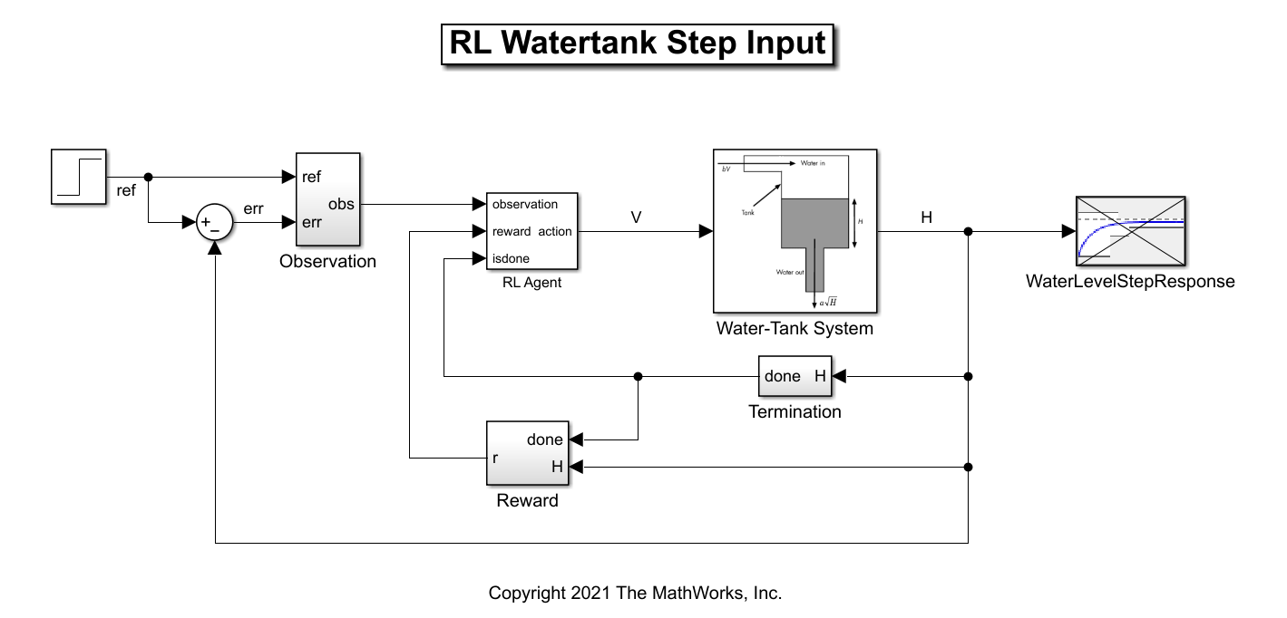

The model in this example has been modified for reinforcement learning. The goal is to control the level of the water in the tank using a reinforcement learning agent, while satisfying the response characteristics defined in the Check Step Response Characteristics block. For more information, see Check Step Response Characteristics (Simulink Design Optimization).

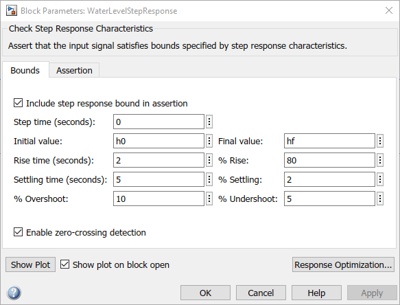
Open the block to view the desired step response specifications.

verifBlk = mdl + "/WaterLevelStepResponse";
open_system(verifBlk)

Generate a Reward Function

Generate the reward function code from specifications in the WaterLevelStepResponse block using generateRewardFunction. The code is displayed in the MATLAB Editor.

generateRewardFunction(blk)

The generated reward function is a starting point for reward design. You may modify the function by choosing different penalty functions and tuning the penalty weights. For this example, make the following change to the generated code:

After you make changes, the weight and penalty specifications should be as follows:

Weight = 10;
Penalty = sum(exteriorPenalty(x,Block1_xmin,Block1_xmax,'quadratic'));

For this example, the modified code has been saved in the MATLAB® function file rewardFunctionVfb.m. Display the generated reward function.

type rewardFunctionVfb.m

function reward = rewardFunctionVfb(x,t)
% REWARDFUNCTION generates rewards 
% from Simulink block specifications.
%
% x : Input of 
% watertank_stepinput_rl/WaterLevelStepResponse
% t : Simulation time (s)

% Reinforcement Learning Toolbox
% 26-Apr-2021 13:05:16

%#codegen

%% Specifications from 
% watertank_stepinput_rl/WaterLevelStepResponse
Block1_InitialValue = 1;
Block1_FinalValue = 2;
Block1_StepTime = 0;
Block1_StepRange = Block1_FinalValue - ...
                   Block1_InitialValue;

Block1_MinRise = Block1_InitialValue + ...
                 Block1_StepRange * 80/100;

Block1_MaxSettling = Block1_InitialValue + ...
                     Block1_StepRange * (1+2/100);

Block1_MinSettling = Block1_InitialValue + ...
                     Block1_StepRange * (1-2/100);

Block1_MaxOvershoot = Block1_InitialValue + ... 
                      Block1_StepRange * (1+10/100);

Block1_MinUndershoot = Block1_InitialValue - ...
                       Block1_StepRange * 5/100;

if t >= Block1_StepTime
    if Block1_InitialValue <= Block1_FinalValue

        Block1_UpperBoundTimes = [0,5; 5,max(5+1,t+1)];

        Block1_UpperBoundAmplitudes = [Block1_MaxOvershoot, ...
                                       Block1_MaxOvershoot; ...
                                       Block1_MaxSettling, ...
                                       Block1_MaxSettling];

        Block1_LowerBoundTimes = [0,2; 2,5; 5,max(5+1,t+1)];

        Block1_LowerBoundAmplitudes = [Block1_MinUndershoot, ...
                                       Block1_MinUndershoot; ...
                                       Block1_MinRise, ...
                                       Block1_MinRise; ...
                                       Block1_MinSettling, ...
                                       Block1_MinSettling];

    else
        
        Block1_UpperBoundTimes = [0,2; 2,5; 5,max(5+1,t+1)];

        Block1_UpperBoundAmplitudes = [Block1_MinUndershoot, ...
                                       Block1_MinUndershoot; ...
                                       Block1_MinRise, ...
                                       Block1_MinRise; ...
                                       Block1_MinSettling, ...
                                       Block1_MinSettling];

        Block1_LowerBoundTimes = [0,5; 5,max(5+1,t+1)];

        Block1_LowerBoundAmplitudes = [Block1_MaxOvershoot, ...
                                       Block1_MaxOvershoot; ...
                                       Block1_MaxSettling, ...
                                       Block1_MaxSettling];
    end

    Block1_xmax = zeros(1,size(Block1_UpperBoundTimes,1));

    for idx = 1:numel(Block1_xmax)
        tseg = Block1_UpperBoundTimes(idx,:);
        xseg = Block1_UpperBoundAmplitudes(idx,:);
        Block1_xmax(idx) = interp1(tseg,xseg,t,'linear',NaN);
    end

    if all(isnan(Block1_xmax))
        Block1_xmax = Inf;
    else
        Block1_xmax = max(Block1_xmax,[],'omitnan');
    end

    Block1_xmin = zeros(1,size(Block1_LowerBoundTimes,1));
    for idx = 1:numel(Block1_xmin)
        tseg = Block1_LowerBoundTimes(idx,:);
        xseg = Block1_LowerBoundAmplitudes(idx,:);
        Block1_xmin(idx) = interp1(tseg,xseg,t,'linear',NaN);
    end
    
    if all(isnan(Block1_xmin))
        Block1_xmin = -Inf;
    else
        Block1_xmin = max(Block1_xmin,[],'omitnan');
    end

else
    Block1_xmin = -Inf;
    Block1_xmax = Inf;
end

%% Penalty function weight (specify nonnegative)
Weight = 10;

%% Compute penalty
% Penalty is computed for violation 
% of linear bound constraints.
%
% To compute exterior bound penalty, 
% use the exteriorPenalty function and
% specify the penalty method 
% as 'step' or 'quadratic'.
%
% Alternaltely, use the hyperbolicPenalty 
% or barrierPenalty function for
% computing hyperbolic and barrier penalties.
%
% For more information, see help for these functions.
Penalty = sum(exteriorPenalty( ...
    x,Block1_xmin,Block1_xmax, ...
    'quadratic'));

%% Compute reward
reward = -Weight * Penalty;
end

To integrate this reward function in the water tank model, open the MATLAB Function block under the Reward Subsystem.

open_system(mdl + "/Reward/Reward Function")

Append the function with the following line of code and save the model.

r = rewardFunctionVfb(x,t);

The MATLAB Function block will now execute rewardFunctionVfb.m for computing rewards.

For this example, the MATLAB Function block has already been modified and saved.

Create a Reinforcement Learning Environment

The environment dynamics are modeled in the Water-Tank Subsystem. For this environment,

Create observation and action specifications for the environment.

numObs = 6;
numAct = 1;
oinfo = rlNumericSpec([numObs 1]);
ainfo = rlNumericSpec([numAct 1]);

Create the reinforcement learning environment using the rlSimulinkEnv function.

agentBlk = mdl + "/RL Agent";
env = rlSimulinkEnv(mdl, agentBlk, oinfo, ainfo);

Create a Reinforcement Learning Agent

Fix the random seed for reproducibility.

rng(0)

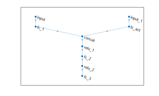
The agent used in this example is a twin-delayed deep deterministic policy gradient (TD3) agent. TD3 agents use two parametrized Q-value function approximators to estimate the value (that is the expected cumulative long-term reward) of the policy. To model the parametrized Q-value function within both critics, use a neural network with two inputs (the observation and action) and one output (the value of the policy when taking a given action from the state corresponding to a given observation). For more information on TD3 agents, see Twin-Delayed Deep Deterministic (TD3) Policy Gradient Agents.

Define each network path as an array of layer objects. Assign names to the input and output layers of each path. These names allow you to connect the paths and then later explicitly associate the network input and output layers with the appropriate environment channel.

% Define paths.
mainPath = [
    featureInputLayer(numObs)
    fullyConnectedLayer(128)
    concatenationLayer(1, 2, Name="concat")
    reluLayer()
    fullyConnectedLayer(128)
    reluLayer()
    fullyConnectedLayer(1)];
actionPath = [
    featureInputLayer(numAct)
    fullyConnectedLayer(8, Name="fc_act")];

% Create dlnetwork object and add layers.
criticNet = dlnetwork();
criticNet = addLayers(criticNet,mainPath);
criticNet = addLayers(criticNet, actionPath);

% Connect Layers.
criticNet = connectLayers(criticNet, "fc_act", "concat/in2");

Plot the critic network structure.

plot(criticNet);

Display the number of weights.

summary(initialize(criticNet));

   Initialized: true

   Number of learnables: 18.5k

   Inputs:
      1   'input'     6 features
      2   'input_1'   1 features

Create the critic function objects using rlQValueFunction. The critic function object encapsulates the critic by wrapping around the critic deep neural network. To make sure the critics have different initial weights, explicitly initialize each network before using them to create the critics.

% Create the two critic functions for the TD3 agent.
critic1 = rlQValueFunction(initialize(criticNet), oinfo, ainfo);
critic2 = rlQValueFunction(initialize(criticNet), oinfo, ainfo);

TD3 agents learn a parametrized deterministic policy over continuous action spaces, which is learned by a continuous deterministic actor. This actor takes the current observation as input and returns as output an action that is a deterministic function of the observation.

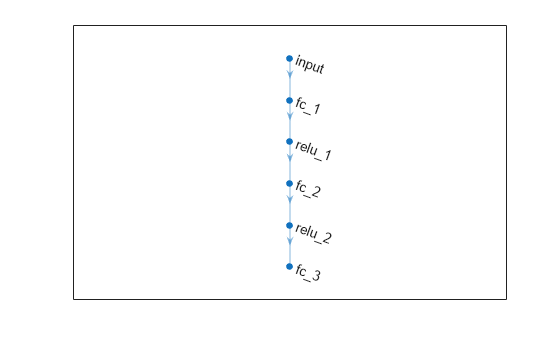
To model the parametrized policy within the actor, use a neural network with one input layer (which receives the content of the environment observation channel, as specified by obsInfo) and one output layer (which returns the action to the environment action channel, as specified by ainfo).

Define the network as an array of layer objects.

actorNet = [
    featureInputLayer(numObs)
    fullyConnectedLayer(128)
    reluLayer()
    fullyConnectedLayer(128)
    reluLayer()
    fullyConnectedLayer(numAct)
    ];

Convert to dlnetwork object, initialize network and display the number of weights.

actorNet = dlnetwork(actorNet);
actorNet = initialize(actorNet);
summary(actorNet)

   Initialized: true

   Number of learnables: 17.5k

   Inputs:
      1   'input'   6 features

Plot the actor network.

plot(actorNet);

Create a deterministic actor function that is responsible for modeling the policy of the agent. For more information, see rlContinuousDeterministicActor.

actordlNet = initialize(actorNet);
actor = rlContinuousDeterministicActor(actordlNet, oinfo, ainfo);

Specify the agent options using rlTD3AgentOptions. The agent trains from an experience buffer of maximum capacity 1e6 by randomly selecting mini-batches of size 256. The discount factor of 0.99 favors long-term rewards.

agentOpts = rlTD3AgentOptions( ...
    SampleTime=Ts, ...
    DiscountFactor=0.99, ...
    ExperienceBufferLength=1e6, ...
    MiniBatchSize=256);

The exploration model in this TD3 agent is Gaussian. The noise model adds a uniform random value to the action during training. Set the standard deviation of the noise to 0.5. Specify the actor and critic optimizer options.

agentOpts.ExplorationModel.StandardDeviation = 0.5;
agentOpts.ActorOptimizerOptions.LearnRate = 1e-3;
agentOpts.ActorOptimizerOptions.GradientThreshold = 1;
agentOpts.CriticOptimizerOptions(1).LearnRate = 1e-3;
agentOpts.CriticOptimizerOptions(1).GradientThreshold = 1;
agentOpts.CriticOptimizerOptions(2).LearnRate = 1e-3;
agentOpts.CriticOptimizerOptions(2).GradientThreshold = 1;

Create the TD3 agent using the actor and critic representations. For more information on TD3 agents, see rlTD3Agent.

agent = rlTD3Agent(actor, [critic1, critic2], agentOpts);

Closed Loop Response

Simulate the model to view the closed loop step response of the untrained agent.

sim(mdl);

Train the Agent

To train the agent, first specify the training options using rlTrainingOptions. For this example, use the following options:

trainOpts = rlTrainingOptions(...
    MaxEpisodes=300, ...
    MaxStepsPerEpisode=ceil(Tf/Ts), ...
    StopTrainingCriteria="EvaluationStatistic",...
    StopTrainingValue=0,...
    ScoreAveragingWindowLength=20);

To evaluate the agent during training, create an rlEvaluator object. Configure the evaluator to run 1 consecutive evaluation episodes every 10 training episodes.

evl = rlEvaluator( ...
    NumEpisodes=1, ...
    EvaluationFrequency=10);

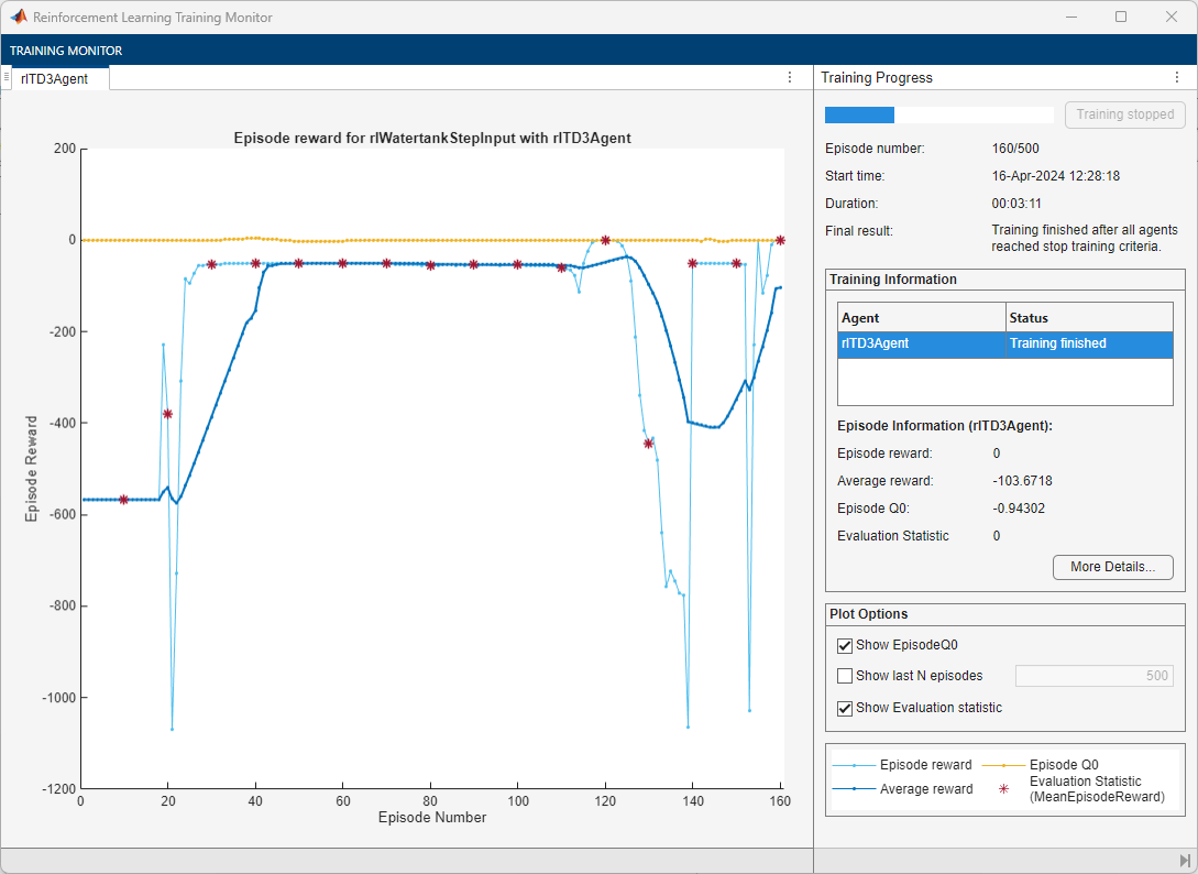
Train the agent using the train function. Training this agent is a computationally intensive process that may take several minutes to complete. To save time while running this example, load a pretrained agent by setting doTraining to false. To train the agent yourself, set doTraining to true.

doTraining = false;
if doTraining
    trainingStats = train(agent, env, trainOpts, Evaluator=evl);
else
    load("rlWatertankTD3Agent.mat")
end

A snapshot of the training progress is shown in the following figure. You can expect different results due to inherent randomness in the training process.

Closed Loop Response of Trained Agent

Simulate the model to view the closed loop step response. The reinforcement learning agent is able to track the reference height while satisfying the step response constraints.

sim(mdl);